QNN: building a quantum classifier

Applicable version · ArcQML 0.1.0

This page highlights the key code paths. Complete programs and data are included with the ArcQML release package. Rust and Python examples can be switched together.

On this page

ArcQML is a quantum machine-learning framework implemented natively in Rust. Its core capabilities include circuit construction, state-vector simulation, observable expectations, automatic differentiation, and parameter optimization. It supports both single and batched quantum states and represents observables using Pauli operators and their linear combinations. Circuit expectations are differentiable tensors that can feed losses and other classical differentiable operations. During backpropagation, gradients traverse the complete graph to circuit parameters. For parameterized circuits, ArcQML uses adjoint differentiation to compute parameter gradients and combines them with classical optimizers such as Adam or SGD to train hybrid quantum–classical algorithms.

These capabilities support variational quantum eigensolvers, quantum neural networks, quantum-state analysis, and small-scale unitary synthesis. Rust provides native compilation, memory safety, and efficient parallelism, allowing ArcQML to combine reliability with strong computational performance.

This tutorial implements a complete binary classification task with ArcQML. It selects 10 features from the German Credit dataset to predict whether an applicant belongs to the bad-credit class. It covers preprocessing, quantum-state encoding, circuit construction and state preparation, binary cross entropy, parameter optimization, validation, and testing. Complete programs are in rust/qnn_german_credit.rs and python/qnn_german_credit.py.

The full dataset is available at data/german_credit.csv.

Preparing the environment

Prepare the release package and environment using Installation and environment setup. Rust users should complete Rust and Runtime configuration; Python users only need wheel installation, without installing Rust or setting Runtime environment variables.

The problem the QNN solves

From classical data to binary predictions

Binary classification is supervised learning of a decision function that assigns each input to one of two mutually exclusive classes. The dataset's Creditability field classifies records as:

0: bad credit, 30% of all records;
1: good credit, 70% of all records.

Here the quantum neural network (QNN) is a parameterized binary classifier. Each record is preprocessed and encoded into a quantum state; all samples then pass through the same trainable circuit. The terminal Pauli-Z expectation of qubit 5 is used as a continuous classification score (logit). Training uses known labels and minimizes binary cross entropy to update circuit parameters, aligning model outputs with the training-label distribution and improving agreement between predicted and true classes.

Data and teaching configuration

Data file: data/german_credit.csv, included with the ArcQML repository.

The German Credit dataset contains 1000 applicant records. Account status, payment history, loan purpose, employment, assets, and other features distinguish good and bad credit. This teaching example uses:

Setting	Value	Purpose
Qubits	10	One qubit per feature.
State-vector length	$2^{10}=1024$	A 10-qubit state contains 1024 complex amplitudes.
QNN layers	1	Controls trainable circuit depth.
Parameters per layer	37	Determined by this rotation-gate structure.
Training / validation / test	800/100/100	Training, development observation, and final evaluation.
Batch size	100	Samples jointly used for each loss and parameter update.
Epochs	5	Five complete passes over the training set.
Adam learning rate	0.01	Controls overall parameter-update magnitude.
Random seed	4	Reproduces data splits and initialization within the same language.

The 10 selected features are Account Balance, Payment Status of Previous Credit, Purpose, Value Savings/Stocks, Length of current employment, Guarantors, Most valuable available asset, Concurrent Credits, Type of apartment, and No of Credits at this Bank, one per qubit.

Initial configuration

First import the interfaces for ArcQML, file reading, and numerical computation:

Rust / Python

use arcqml::prelude::*;
use num_complex::Complex64;
use std::{f64::consts::PI, fs};

// `AppResult<T>` returns T on success and a printable error on failure.
// The `?` below propagates errors to the caller.
type AppResult<T> = std::result::Result<T, Box<dyn std::error::Error>>;

from __future__ import annotations

import csv
from pathlib import Path

import numpy as np
import arcqml

The main numerical settings are declared together as constants:

Rust / Python

const QUBITS: usize = 10;                   // Ten features correspond to ten qubits
const STATE_DIMENSION: usize = 1 << QUBITS; // That is, 2^10 = 1024
const PARAMETERS_PER_LAYER: usize = 37;     // Determined by the circuit structure declared below
const LAYERS: usize = 1;                    // Use only one layer to keep the tutorial fast
const EPOCHS: usize = 5;                    // Complete five passes over the training set
const BATCH_SIZE: usize = 100;              // Process 100 records at a time
const LEARNING_RATE: f64 = 0.01;            // Adam learning rate
const SEED: u64 = 4;                        // Fixed seed for reproducibility
const DATA_PATH: &str = "data/german_credit.csv";

QUBITS = 10                    # Ten features correspond to ten qubits
STATE_DIMENSION = 1 << QUBITS  # That is, 2**10 = 1024
PARAMETERS_PER_LAYER = 37      # Determined by the circuit structure declared below.
LAYERS = 1                     # Use only one layer to keep the tutorial fast
EPOCHS = 5                     # Complete five passes over the training set
BATCH_SIZE = 100               # Process 100 records at a time
LEARNING_RATE = 0.01           # Adam learning rate
SEED = 4                       # Fixed seed for reproducibility
DATA_PATH = Path(__file__).resolve().parents[1] / "data" / "german_credit.csv"

Some hyperparameters can be adjusted in later experiments.

Loading and preprocessing data

Reading labels

In Creditability, 1 denotes good credit and 0 bad credit. This example instead uses bad credit as positive class 1:

Rust / Python

// Read the label column.
let label_column = headers
    .iter()
    .position(|name| *name == "Creditability")
    .ok_or("missing Creditability column")?;

let creditability: u8 = fields[label_column].parse()?;

// Map 1 (good credit) to label 0 and 0 (bad credit) to label 1.
let label = f64::from(1 - creditability);

labels = np.asarray(
    [1.0 - float(row["Creditability"]) for row in rows],
    dtype=np.float64,
)

Preprocessing features

Raw features are discrete numerical values and should not be used directly as rotation angles. The example independently applies min-max scaling to each feature column:

x'=\frac{\pi}{2}+\frac{x-x_{\min}}{x_{\max}-x_{\min}}\pi.

Here $x_{\min}$ and $x_{\max}$ are the minimum and maximum of the feature over all 1000 records. After transformation, each value lies in $[\pi/2,3\pi/2]$ and can directly serve as an RX or RZ rotation angle.

Rust / Python

for column in 0..QUBITS {
    let minimum = samples
        .iter()
        .map(|sample| sample.features[column])
        .fold(f64::INFINITY, f64::min);
    let maximum = samples
        .iter()
        .map(|sample| sample.features[column])
        .fold(f64::NEG_INFINITY, f64::max);

    for sample in &mut samples {
        // Scale this feature column to [π/2, 3π/2] to obtain radians for angle encoding.
        sample.features[column] =
            PI / 2.0
            + (sample.features[column] - minimum) / (maximum - minimum) * PI;
    }
}

minimum = features.min(axis=0)
maximum = features.max(axis=0)

# Scale this feature column to [π/2, 3π/2] to obtain radians for angle encoding.
features = (
    np.pi / 2.0
    + (features - minimum) / (maximum - minimum) * np.pi
)

A constant column would give $x_{\max}-x_{\min}=0$ . None of the 10 selected columns is constant. If replacing features, check for and remove constant columns, or assign them a fixed encoding angle.

Splitting the dataset

The program shuffles records, then splits training, validation, and test sets in an 8:1:1 ratio:

Rust / Python

Rng::new(SEED).shuffle(&mut samples);
let test_samples = samples.split_off(900);        // Test set
let validation_samples = samples.split_off(800);  // Validation set
let training_samples = samples;                   // Training set

rng = np.random.default_rng(seed=SEED)
shuffled_indices = rng.permutation(len(features))
training_indices = shuffled_indices[:800]         # Training set
validation_indices = shuffled_indices[800:900]    # Validation set
test_indices = shuffled_indices[900:]             # Test set

Preparing initial quantum states

Angle encoding

Each record contains 10 scaled angles $x'_0,x'_1,\ldots,x'_9$ . On qubit $i$ , the example applies RX(x'_i) followed by RZ(x'_i). Using classical values as quantum-gate angles is called angle encoding.

Starting from $\lvert0\rangle$ , a single encoded qubit is:

R_Z(x')R_X(x')\lvert0\rangle= e^{-ix'/2}\cos(x'/2)\lvert0\rangle -i e^{ix'/2}\sin(x'/2)\lvert1\rangle.

The 10 qubits are unentangled during encoding, so a record becomes the tensor product of 10 local states. Each record yields a complex state vector of length $2^{10}=1024$ .

Preparing quantum states

Adding RX(x'_i) and RZ(x'_i) directly to the trainable circuit would also register their angles as ArcQML parameters. To avoid this, the example precomputes exactly equivalent encoded states, then shares one circuit containing only the 37 trainable parameters across all samples.

Rust / Python

fn encode_product_states(samples: &[Sample]) -> AppResult<Tensor> {
    let mut encoded_amplitudes =
        Vec::with_capacity(samples.len() * STATE_DIMENSION);

    for sample in samples {
        let mut encoded_state = vec![Complex64::new(1.0, 0.0)];

        // Expand in q9, q8, ..., q0 order so the final amplitude indices match ArcQML.
        for qubit in (0..QUBITS).rev() {
            let angle = sample.features[qubit];
            let half_angle = angle / 2.0;
            let amplitude_zero =
                Complex64::from_polar(1.0, -half_angle) * half_angle.cos();
            let amplitude_one = Complex64::new(0.0, -1.0)
                * Complex64::from_polar(1.0, half_angle)
                * half_angle.sin();

            let mut expanded_state = Vec::with_capacity(encoded_state.len() * 2);
            for amplitude in encoded_state {
                expanded_state.push(amplitude * amplitude_zero);
                expanded_state.push(amplitude * amplitude_one);
            }
            encoded_state = expanded_state;
        }
        encoded_amplitudes.extend(encoded_state);
    }

    Ok(Tensor::new(TensorData::FlatC64 {
        data: encoded_amplitudes,
        shape: vec![samples.len(), STATE_DIMENSION],
    })?)
}

def encode_product_states(features: np.ndarray) -> np.ndarray:
    """Convert angle encoding directly into a batch of product states."""
    encoded_states = np.ones((len(features), 1), dtype=np.complex128)

    # Expand in q9, q8, ..., q0 order so the final amplitude indices match ArcQML.
    for qubit in range(QUBITS - 1, -1, -1):
        angles = features[:, qubit]
        local_encoded_states = np.column_stack(
            (
                np.exp(-0.5j * angles) * np.cos(0.5 * angles),
                -1j * np.exp(0.5j * angles) * np.sin(0.5 * angles),
            )
        )
        encoded_states = np.einsum(
            "bi,bj->bij",
            encoded_states,
            local_encoded_states,
        ).reshape(len(features), -1)

    assert encoded_states.shape == (len(features), STATE_DIMENSION)
    return np.ascontiguousarray(encoded_states, dtype=np.complex128)

Each record produces an encoded quantum state. Collecting these into shape [number of samples, 1024] gives a batched quantum-state array.

Constructing the variational circuit

Single-layer circuit structure

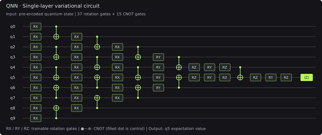
Angle encoding inserts the input data; the optimizer updates only trainable parameters in the variational circuit. This example has 1 layer, containing 37 rotation gates and 15 CNOT gates, for 52 gates total. Rotations provide trainable angles; CNOTs correlate qubits. Adjust LAYERS to change the layer count.

Rust / Python

fn append_ansatz_layer(circuit: &mut Circuit, values: &[f64]) -> AppResult<()> {
    if values.len() != PARAMETERS_PER_LAYER {
        return Err("each ansatz layer requires 37 parameters".into());
    }
    for qubit in 0..QUBITS {
        circuit.rx(values[qubit], qubit)?;
    }
    for (control, target) in [(0, 1), (2, 3), (4, 5), (9, 8), (7, 6)] {
        circuit.cnot(control, target)?;
    }
    for qubit in 1..9 {
        circuit.rx(values[9 + qubit], qubit)?;
    }
    for (control, target) in [(1, 2), (3, 4), (8, 7), (6, 5)] {
        circuit.cnot(control, target)?;
    }
    for qubit in 2..8 {
        circuit.rx(values[16 + qubit], qubit)?;
    }
    for (control, target) in [(2, 3), (4, 5), (7, 6)] {
        circuit.cnot(control, target)?;
    }
    for (parameter, qubit) in [(24, 3), (25, 4), (26, 5), (27, 6)] {
        circuit.ry(values[parameter], qubit)?;
    }
    circuit.cnot(3, 4)?.cnot(6, 5)?;
    circuit
        .rz(values[28], 4)?
        .ry(values[29], 4)?
        .rz(values[30], 4)?;
    circuit
        .rz(values[31], 5)?
        .ry(values[32], 5)?
        .rz(values[33], 5)?;
    circuit.cnot(4, 5)?;
    circuit
        .rz(values[34], 5)?
        .ry(values[35], 5)?
        .rz(values[36], 5)?;
    Ok(())
}

def append_ansatz_layer(circuit: arcqml.Circuit, values: np.ndarray) -> None:
    if values.shape != (PARAMETERS_PER_LAYER,):
        raise ValueError("each ansatz layer requires 37 parameters")
    for qubit in range(QUBITS):
        circuit.rx(angle=float(values[qubit]), qubit=qubit)
    for control, target in ((0, 1), (2, 3), (4, 5), (9, 8), (7, 6)):
        circuit.cnot(control=control, target=target)
    for qubit in range(1, 9):
        circuit.rx(angle=float(values[9 + qubit]), qubit=qubit)
    for control, target in ((1, 2), (3, 4), (8, 7), (6, 5)):
        circuit.cnot(control=control, target=target)
    for qubit in range(2, 8):
        circuit.rx(angle=float(values[16 + qubit]), qubit=qubit)
    for control, target in ((2, 3), (4, 5), (7, 6)):
        circuit.cnot(control=control, target=target)
    for parameter, qubit in ((24, 3), (25, 4), (26, 5), (27, 6)):
        circuit.ry(angle=float(values[parameter]), qubit=qubit)
    circuit.cnot(control=3, target=4)
    circuit.cnot(control=6, target=5)
    circuit.rz(angle=float(values[28]), qubit=4)
    circuit.ry(angle=float(values[29]), qubit=4)
    circuit.rz(angle=float(values[30]), qubit=4)
    circuit.rz(angle=float(values[31]), qubit=5)
    circuit.ry(angle=float(values[32]), qubit=5)
    circuit.rz(angle=float(values[33]), qubit=5)
    circuit.cnot(control=4, target=5)
    circuit.rz(angle=float(values[34]), qubit=5)
    circuit.ry(angle=float(values[35]), qubit=5)
    circuit.rz(angle=float(values[36]), qubit=5)

The circuit is shown below; scroll horizontally to see it in full:

A single-layer, 10-qubit QNN with 37 rotation gates and 15 CNOT gates, followed by measurement of the Pauli-Z expectation on q5

Initializing angles

The example draws 37 trainable angles from the standard normal distribution, with mean 0 and standard deviation 1.

Rust / Python

let mut rng = Rng::new(SEED);

// Create the circuit
let mut circuit = Circuit::new(QUBITS)?;

for _layer in 0..LAYERS {
    // Generate standard-normal initial values
    let initial_angles: Vec<f64> = (0..PARAMETERS_PER_LAYER)
        .map(|_| rng.normal())
        .collect();
    append_ansatz_layer(&mut circuit, &initial_angles)?;
}

rng = np.random.default_rng(seed=SEED)

# Create the circuit
circuit = arcqml.Circuit(num_qubits=QUBITS)

for _layer in range(LAYERS):
    # Generate standard-normal initial values
    initial_angles = rng.standard_normal(PARAMETERS_PER_LAYER)
    append_ansatz_layer(circuit=circuit, values=initial_angles)

Measuring the expectation

The example measures the Pauli-Z expectation of qubit 5. The choice of q5 is fixed by this circuit design because it aggregates information from all features.

Rust / Python

let observable = SparsePauliOp::single(
    QUBITS,
    5usize,  // Measure q5
    Pauli::Z,
    1.0,     // Coefficient of the Pauli-Z term
)?;

observable = arcqml.PauliSum.z(
    num_qubits=QUBITS,
    qubit=5,            # Measure q5
    coefficient=1.0,    # Coefficient of the Pauli-Z term
)

For sample $i$ , the model output is:

z_i= \langle\psi(x'_i,\boldsymbol{\theta})\rvert Z_5 \lvert\psi(x'_i,\boldsymbol{\theta})\rangle.

Here $x'_i$ denotes the encoded input features and $\boldsymbol{\theta}$ the trainable circuit angles. The Pauli-Z expectation lies in $[-1,1]$ . The example uses $z_i$ directly as a binary logit and interprets its sigmoid as the positive-class probability:

p_i=\sigma(z_i)=\frac{1}{1+e^{-z_i}}.

$z_i\ge0$ is equivalent to $p_i\ge0.5$ , predicting bad credit; $z_i<0$ predicts good credit.

Defining the loss

A loss summarizes predictions and known labels as one value to minimize. This example uses binary cross entropy with logits. For a batch of $N$ records:

\mathcal{L}=-\frac{1}{N}\sum_{i=1}^{N} \left[ y_i\log\sigma(z_i) +(1-y_i)\log\left(1-\sigma(z_i)\right) \right].

If $y_i=1$ , the loss pushes $z_i$ upward; if $y_i=0$ , it pushes $z_i$ downward.

Rust / Python

let targets = labels(training_samples)?;
let loss = binary_cross_entropy_with_logits_loss(
    &logits,
    &targets,
)?;

// The loss is the mean binary cross-entropy over the batch, not one sample loss
let loss_value = loss.value()?;

targets = arcqml.tensor(
    np.ascontiguousarray(training_labels, dtype=np.float64)
)
loss = arcqml.binary_cross_entropy_with_logits(
    logits=logits,
    targets=targets,
)

# The loss is the mean binary cross-entropy over the batch, not one sample loss
loss_value = float(loss.item())

Lower loss means closer agreement between predictions and labels. Iteratively optimizing trainable circuit parameters to minimize the loss moves classification scores toward their label targets, improving the model ability to predict sample classes.

Creating the simulator and optimizer

State-vector simulator

Rust / Python

// Create a simulator from the given state.
let simulator = BatchStateVectorSimulator::from_state_tensor(QUBITS, states)?;

# Create a simulator from the given state.
simulator = arcqml.BatchStateVectorSimulator.from_amplitudes(
                num_qubits=QUBITS,
                amplitudes=np.ascontiguousarray(states[batch_indices]),
            )

The simulator executes the full circuit from the supplied states. Neither Rust simulator.run(circuit, observable) nor Python simulator.run(circuit=circuit, observable=observable) permanently changes the stored initial states, so one simulator can be reused throughout training.

Adam optimizer

Ordinary gradient descent uses one fixed update scale for all parameters. Adam tracks recent averages of gradients and squared gradients separately for each parameter, adapting its effective update magnitude.

Rust / Python

let mut optimizer = Adam::new(
    LEARNING_RATE, // Use the previously defined learning rate of 0.01
    0.9,   // beta1
    0.999, // beta2
    1e-8,  // epsilon
    0.0,   // weight_decay
)?;

# Other optional parameters use the same defaults as the Rust example.
optimizer = arcqml.Adam(learning_rate=LEARNING_RATE)

These hyperparameters are not suitable for every task and circuit. Retune them if training performs poorly.

Batch forward passes and backpropagation

Each training iteration has four steps:

Evaluate the current loss in a forward pass.
Backpropagate from the loss to obtain all parameter gradients.
Update parameters with Adam.
Clear the current gradients to prevent accumulation with the next iteration.

Rust / Python

// Pseudocode for illustration only.

// logits has shape [batch size]; each entry is one record's Z(q5) expectation.
let logits = simulator.run(circuit, observable)?;

// Compute the current loss in the forward pass.
let loss = binary_cross_entropy_with_logits_loss(&logits, &targets)?;

// Backpropagate from the loss to compute all parameter gradients.
loss.backward()?;

// Adam updates parameters using the gradients.
optimizer.step(circuit.parameters())?;

// Clear current gradients to prevent accumulation in the next iteration.
optimizer.zero_grad(circuit.parameters());

# Pseudocode for illustration only.

# logits has shape [batch size]; each entry is one record's Z(q5) expectation.
logits = simulator.run(circuit=circuit, observable=observable)

# Compute the current loss in the forward pass.
loss = arcqml.binary_cross_entropy_with_logits(
    logits=logits,
    targets=targets,
)

# Backpropagate from the loss to compute all parameter gradients.
loss.backward()

# Adam updates parameters using the gradients.
optimizer.step(circuit=circuit)

# Clear current gradients to prevent accumulation in the next iteration.
optimizer.zero_grad(circuit=circuit)

run returns a Tensor; when backward() is called, ArcQML uses the recorded graph to compute gradients. Parameters have no gradients before the first iteration, so no initial zero_grad is needed. After the first backward pass, clear gradients every iteration.

Validation and testing

Validation and testing read outputs without updating parameters, so disable gradient recording to reduce unnecessary graph storage and memory use:

Rust / Python

let _guard = no_grad();
let encoded_states = encode_product_states(evaluation_samples)?;
let simulator = BatchStateVectorSimulator::from_state_tensor(
    QUBITS,
    encoded_states,
)?;
let logits = simulator.run(&circuit, &observable)?;

// Gradient recording resumes when `_guard` leaves this scope.

encoded_state_batch = np.ascontiguousarray(
    evaluation_encoded_states,
    dtype=np.complex128,
)
simulator = arcqml.BatchStateVectorSimulator.from_amplitudes(
    num_qubits=QUBITS,
    amplitudes=encoded_state_batch,
)

with arcqml.no_grad():
    scores = simulator.run(
        circuit=circuit,
        observable=observable,
    ).numpy()

Running the complete example

Rust version

In the Rust setup instructions, you set ARCQML_RUNTIME_LIB_DIR; use that same Windows PowerShell or Linux terminal to run:

text

cargo run --release -p arcqml --example qnn_german_credit

Python version

Install the wheel and activate the Conda environment as in the Python setup instructions, then run from the ArcQML root:

text

conda activate arcqml-example
python python/qnn_german_credit.py

Example output

Both programs display the data split, parameter count, training and validation results per epoch, and final test-set AUC:

text

samples: train=800, validation=100, test=100
qubits=10, layers=1, parameters=37
epoch 01/5: train_loss=..., validation_loss=..., validation_accuracy=...%
...
epoch 05/5: train_loss=..., validation_loss=..., validation_accuracy=...%
test ROC-AUC=..., PR-AUC=...

Interpreting the results

An overall decrease in training loss indicates learning. Small epoch-to-epoch fluctuations are normal with minibatches and Adam.
Falling training and validation losses usually indicate healthy progress. If training loss falls while validation loss keeps rising, the model may be overfitting.
With only 100 validation and 100 test records, metrics may vary substantially with the split. One run is not a production conclusion.
A 10-qubit state vector contains 1024 complex amplitudes. Memory and computation grow as $2^n$ with the qubit count. Evaluate costs before adding features or layers.

Next steps

Try extending the example:

Adjust EPOCHS, BATCH_SIZE, or the Adam learning rate and observe training stability and validation performance.
Increase LAYERS from 1 to 2 and compare the expressive capacity and cost of more parameters.
Save trained circuit parameters, then restore and evaluate them in a separate test program.

Download Markdown tutorial ↓