VQE: solving the H₂ ground-state energy
Applicable version · ArcQML 0.1.0
This page highlights the key code paths. Complete programs and data are included with the ArcQML release package. Rust and Python examples can be switched together.
On this page
ArcQML is a quantum machine-learning framework implemented natively in Rust. Its core capabilities include circuit construction, state-vector simulation, observable expectations, automatic differentiation, and parameter optimization. It supports both single and batched quantum states and represents observables using Pauli operators and their linear combinations. Circuit expectations are differentiable tensors that can feed losses and other classical differentiable operations. During backpropagation, gradients traverse the complete graph to circuit parameters. For parameterized circuits, ArcQML uses adjoint differentiation to compute parameter gradients and combines them with classical optimizers such as Adam or SGD to train hybrid quantum–classical algorithms.
These capabilities support variational quantum eigensolvers, quantum neural networks, quantum-state analysis, and small-scale unitary synthesis. Rust provides native compilation, memory safety, and efficient parallelism, allowing ArcQML to combine reliability with strong computational performance.
This tutorial implements a complete variational quantum eigensolver (VQE) in ArcQML to estimate the H₂ ground-state energy for a specified geometry, basis set, and active space. It explains how to map an electronic-structure problem to a qubit Hamiltonian, construct a circuit and prepare states, evaluate energy, obtain gradients, and update parameters. Complete programs are in rust/h2_vqe.rs and python/h2_vqe.py.
Preparing the environment
Prepare the release package and environment using Installation and environment setup. Rust users should complete Rust and Runtime configuration; Python users only need wheel installation, without installing Rust or setting Runtime environment variables.
The problem VQE solves
Complete computation workflow
A molecule can occupy states with different energies; the lowest-energy state is its ground state. Ground-state energy is fundamental to predicting molecular stability, chemical reactions, and material properties. As systems grow, the storage and computation needed to find the lowest energy of large molecules directly on a classical computer increase exponentially. A variational quantum eigensolver (VQE) uses a quantum device to prepare parameterized states and measure energy expectations, and a classical computer to update circuit parameters. This hybrid approach avoids the huge cost of storing and diagonalizing the full high-dimensional matrix classically.
VQE is a hybrid quantum–classical algorithm for estimating a quantum-system ground-state energy. For Hamiltonian with smallest eigenvalue , the variational principle gives, for any normalized state :
With parameters , construct a circuit . Choose an easily prepared reference state and evolve it into a parameterized state :
In quantum chemistry, the electronic Hamiltonian is usually written in second-quantized form using fermionic creation and annihilation operators. After selecting active electrons and orbitals, a fermion-to-qubit mapping such as Jordan–Wigner transforms it into a qubit Hamiltonian:
Here are real coefficients and are Pauli strings composed of X, Y, Z, and identity operators. The objective is the Hamiltonian energy expectation in the parameterized state:
A classical optimizer iteratively updates parameters from measurement results to reduce . The minimum found is a variational upper bound on . If the circuit can represent the ground state and optimization converges sufficiently, the result can approach the true ground-state energy.
Chemistry settings
This example uses the following quantum-chemistry settings:
| Setting | Value |
|---|---|
| Molecular geometry | H (0, 0, -0.35 Å), H (0, 0, 0.35 Å) |
| Interatomic distance | 0.70 Å |
| Basis set | STO-3G |
| Active electrons | 2 |
| Active orbitals | 2 |
| Fermionic mapping | Jordan–Wigner |
| Qubits | 4 |
| Hamiltonian terms | 15 |
| Fixed-particle-number subspace dimension | 6 |
| Hartree–Fock energy | -1.1173490350562805 Ha |
| Exact ground-state energy | -1.1361894542078266 Ha |
Initial configuration
First import the required ArcQML and standard-library interfaces:
use arcqml::prelude::*;

// `AppResult<T>` returns T when the function succeeds and a printable error on failure.
// The `?` below propagates errors to the caller.
type AppResult<T> = std::result::Result<T, Box<dyn std::error::Error>>;
from __future__ import annotations

import json
import math
from pathlib import Path

import arcqml
The main numerical settings are declared together as constants:
const NUM_QUBITS: usize = 4;       // The H₂ mapping requires 4 qubits
const ACTIVE_ELECTRONS: usize = 2; // The Hartree–Fock initial state occupies the first two positions
const LAYERS: usize = 6;           // Repeat the trainable circuit for six layers
const STEPS: usize = 100;          // Update parameters 100 times

const EXACT_GROUND_ENERGY: f64 = -1.136_189_454_207_826_6;    // Exact ground-state energy
const HARTREE_FOCK_ENERGY: f64 = -1.117_349_035_056_280_5;    // Hartree–Fock energy (initial-state energy)

const CHEMICAL_ACCURACY: f64 = 1.6e-3;    // Chemical-accuracy error threshold
NUM_QUBITS = 4       # The H₂ mapping requires 4 qubits
ACTIVE_ELECTRONS = 2 # The Hartree–Fock initial state occupies the first two positions
LAYERS = 6           # Repeat the trainable circuit for six layers
STEPS = 100          # Update parameters 100 times

EXACT_GROUND_ENERGY = -1.136_189_454_207_826_6    # Exact ground-state energy
HARTREE_FOCK_ENERGY = -1.117_349_035_056_280_5    # Hartree–Fock energy (initial-state energy)

CHEMICAL_ACCURACY = 1.6e-3    # Chemical-accuracy error threshold
The layer and training-step counts are example hyperparameters that can be adjusted in later experiments.
Constructing the Hamiltonian
The Hamiltonian was generated with the third-party quantum-computing tool PennyLane. After the Jordan–Wigner transform, H₂ has a real-coefficient linear combination of 15 Pauli strings. ArcQML stores these terms in Rust SparsePauliOp or Python PauliSum. Pauli X, Y, and Z are basic operators for single-qubit transformations or measurements; their weighted sum represents the molecular energy here. Rust reads the JSON at compile time with include_str!, while Python reads it at runtime and constructs each term:
let hamiltonian = SparsePauliOp::from_json(include_str!(
    "../data/h2_hamiltonian.json"
))?;

// Ensure the imported Hamiltonian has 4 qubits and 15 terms
assert_eq!(hamiltonian.num_qubits(), 4);
assert_eq!(hamiltonian.len(), 15);
DATA_PATH = Path(__file__).resolve().parents[1] / "data" / "h2_hamiltonian.json"


def load_hamiltonian(path: Path) -> arcqml.PauliSum:
    # The public Python API cannot yet load JSON directly, so build the PauliSum term by term.
    payload = json.loads(path.read_text(encoding="utf-8"))
    hamiltonian = arcqml.PauliSum(num_qubits=payload["num_qubits"])

    for term in payload["terms"]:
        coefficient = term["coefficient"]
        operations = term["paulis"]
        if not operations:
            # Identity operator
            hamiltonian.add_identity(coefficient=coefficient)
            continue
        hamiltonian.add_term(
            paulis="".join(operation["pauli"] for operation in operations),
            qubits=[operation["qubit"] for operation in operations],
            coefficient=coefficient,
        )
    return hamiltonian


hamiltonian = load_hamiltonian(path=DATA_PATH)
# Ensure the imported Hamiltonian has 4 qubits and 15 terms
assert hamiltonian.num_qubits == 4
assert hamiltonian.num_terms == 15
ArcQML JSON has top-level num_qubits and terms fields. Each Pauli operation explicitly records qubit and pauli. For example, the constant term and X(q0)X(q1)Y(q2)Y(q3) term are:
{
  "num_qubits": 4,
  "terms": [
    {
      "coefficient": -0.042078985845795724,
      "paulis": []
    },
    {
      "coefficient": -0.04475014386992153,
      "paulis": [
        { "qubit": 0, "pauli": "X" },
        { "qubit": 1, "pauli": "X" },
        { "qubit": 2, "pauli": "Y" },
        { "qubit": 3, "pauli": "Y" }
      ]
    }
  ]
}
An empty paulis array denotes the identity operator.
Preparing the initial quantum state
Circuit::new(4) creates a four-qubit circuit. The simulator starts in , with all four positions unoccupied. Under Jordan–Wigner mapping, the two active electrons here occupy the two lowest-numbered positions, so X gates on qubits 0 and 1 flip those bits from 0 to 1:
let mut circuit = Circuit::new(NUM_QUBITS)?;

// Apply X gates to qubits 0 and 1 in order
for qubit in 0..ACTIVE_ELECTRONS {
    circuit.x(qubit)?;
}
circuit = arcqml.Circuit(num_qubits=NUM_QUBITS)

# Apply X gates to qubits 0 and 1 in order
for qubit in range(ACTIVE_ELECTRONS):
    circuit.x(qubit=qubit)
ArcQML displays state strings in descending qubit order, . Setting qubits 0 and 1 to 1 therefore displays .
Constructing the variational circuit
Initializing angles
The initialization formula is:
Here 0.04 is the angular amplitude in radians. It restricts every initial rotation angle to , avoiding large single-qubit rotations at the start. The fixed phase increment 0.37 gives neighboring parameters different asymmetric initial values, rather than setting all 48 angles identically. The sine function varies angles smoothly with parameter index and produces both signs.
Building the circuit
The example uses 6 layers of a hardware-efficient parameterized circuit. Each layer applies RY and RZ to every qubit, then a ring of CNOT entanglers:
let mut parameter_index = 0usize;

for _layer in 0..LAYERS {
    for qubit in 0..NUM_QUBITS {
        // Initialize angles
        let ry = 0.04 * (0.37 * (parameter_index + 1) as f64).sin();
        parameter_index += 1;

        let rz = 0.04 * (0.37 * (parameter_index + 1) as f64).sin();
        parameter_index += 1;

        // The ry and rz functions register their angles as trainable parameters.
        circuit.ry(ry, qubit)?;
        circuit.rz(rz, qubit)?;
    }

    for control in 0..NUM_QUBITS {
        // Ring of CNOT entangling gates.
        let target = (control + 1) % NUM_QUBITS;
        circuit.cnot(control, target)?;
    }
}
parameter_index = 0

for _layer in range(LAYERS):
    for qubit in range(NUM_QUBITS):
        # Initialize angles
        ry = 0.04 * math.sin(0.37 * (parameter_index + 1))
        parameter_index += 1

        rz = 0.04 * math.sin(0.37 * (parameter_index + 1))
        parameter_index += 1

        # The ry and rz functions register their angles as trainable parameters.
        circuit.ry(angle=ry, qubit=qubit)
        circuit.rz(angle=rz, qubit=qubit)

    for control in range(NUM_QUBITS):
        # Ring of CNOT entangling gates.
        circuit.cnot(
            control=control,
            target=(control + 1) % NUM_QUBITS,
        )
The circuit structure is shown below:
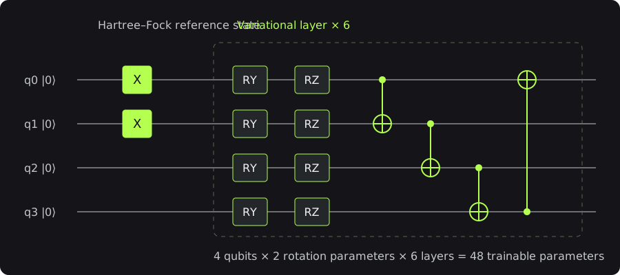
This hardware-efficient circuit does not strictly preserve particle number. It demonstrates general VQE and ArcQML autograd. Chemistry applications can instead use particle-number-preserving excitation circuits.
Creating the simulator and optimizer
State-vector simulator
let simulator = StateVectorSimulator::new(NUM_QUBITS)?;
simulator = arcqml.StateVectorSimulator(num_qubits=NUM_QUBITS)
The simulator executes the complete circuit from . Hartree–Fock preparation gates are placed first, so every evaluation prepares before applying the trainable circuit.
Neither Rust simulator.run(&circuit, &hamiltonian) nor Python simulator.run(circuit=circuit, observable=hamiltonian) permanently changes the stored initial state. One simulator can therefore be reused throughout training.
Adam optimizer
Ordinary gradient descent uses one fixed update scale for all parameters. Adam tracks recent averages of gradients and squared gradients separately for each parameter, adapting its effective update magnitude.
let mut optimizer = Adam::new(
    0.05,  // Learning rate
    0.9,   // beta1
    0.999, // beta2
    1e-8,  // epsilon
    0.0,   // weight_decay
)?;
# Other optional parameters use the same defaults as the Rust example.
optimizer = arcqml.Adam(learning_rate=0.05)
These hyperparameters are not suitable for every molecule and circuit. Retune them if training performs poorly.
Running VQE optimization
Each training iteration has four steps:
- Evaluate the current energy in a forward pass.
- Backpropagate from the energy to obtain gradients of all 48 parameters.
- Update parameters with Adam.
- Clear the current gradients to prevent accumulation with the next iteration.
for step in 1..=STEPS {
    // Compute the current energy in the forward pass.
    let energy = simulator.run(&circuit, &hamiltonian)?;

    // Compute gradients for all trainable angles in the backward pass
    energy.backward()?;

    // The optimizer reads gradients and updates parameters
    optimizer.step(circuit.parameters())?;

    // Clear the current gradients.
    optimizer.zero_grad(circuit.parameters());

    // Print the updated energy at step 1 and every 10 steps thereafter.
    if step == 1 || step % 10 == 0 {
        let current = simulator.run(&circuit, &hamiltonian)?.value()?;
        println!("step {step:>3}: energy = {current:.12} Ha");
    }
}
for step in range(1, STEPS + 1):
    # Compute the current energy in the forward pass.
    energy_tensor = simulator.run(circuit=circuit, observable=hamiltonian)

    # Compute gradients for all trainable angles in the backward pass
    energy_tensor.backward()

    # The optimizer reads gradients and updates parameters
    optimizer.step(circuit=circuit)

    # Clear the current gradients.
    optimizer.zero_grad(circuit=circuit)

    # Print the updated energy at step 1 and every 10 steps thereafter.
    if step == 1 or step % 10 == 0:
        with arcqml.no_grad():
            current = simulator.run(
                circuit=circuit,
                observable=hamiltonian,
            ).item()
        print(f"step {step:>3}: energy = {current:.12f} Ha")
run returns a Tensor; when backward() is called, ArcQML uses the recorded graph to compute gradients. Parameters have no gradients before the first iteration, so no initial zero_grad is needed. After the first backward pass, clear gradients every iteration.
Running the complete example
Rust version
In the Rust setup instructions, you set ARCQML_RUNTIME_LIB_DIR; use that same Windows PowerShell or Linux terminal to run:
cargo run --release -p arcqml --example h2_vqe
Python version
Install the wheel and activate the Conda environment as in the Python setup instructions, then run from the ArcQML root:
conda activate arcqml-example
python python/h2_vqe.py
Example output
Every 10 steps, the program prints the energy and its absolute error against the exact ground-state energy. It finally checks whether chemical accuracy has been reached:
H2/STO-3G, Jordan-Wigner, 4 qubits
Hamiltonian terms : 15
Trainable params  : 48
Hartree-Fock      : -1.117349035056 Ha
Exact ground      : -1.136189454208 Ha
step   1: energy = -0.401257301811 Ha, |error| = 7.349e-1 Ha
...
step 100: energy = -1.136145412038 Ha, |error| = 4.404e-5 Ha

VQE energy        : -1.136145412038 Ha
Absolute error    : 4.404217e-5 Ha
Chemical accuracy: reached (threshold 1.6e-3 Ha)
Interpreting the results
- Energy should generally converge downward from its initial value and, under the variational principle, should not fall substantially below the exact ground-state energy.
- The Hartree–Fock to exact-energy gap is about
0.0188404 Ha, mainly due to electron correlation. - An absolute error below
1.6 × 10⁻³ Hais commonly called chemical accuracy. - If 100 steps are insufficient, increase training steps, tune the learning rate, or add circuit layers. Deeper circuits can also increase optimization plateaus or parameter redundancy.
Next steps
Try extending the example:
- Replace
AdamwithSgdand compare convergence speed. - Use particle-number-preserving excitation circuits to restrict search to the 6-dimensional two-electron subspace.
- Save trained circuit weights and restore them in a new process with
load_weights. - Vary the H–H bond length to compute a potential-energy curve.